
Building AI Shadow Profiler: How I Prototyped a Behavioral Classifier in a 100-Minute Lab Session
An engineering story about Bayesian inference, psychophysiology, synthetic data, and the journey from a classroom concept to a working Python prototype.
Author: CODERUDRA-X
Category: Artificial Intelligence · Machine Learning · Engineering
Tech stack: Python · NumPy · Pandas · Scikit-learn · Jupyter Notebook
Project stage: Experimental prototype · Synthetic data only
Scope note: The code in this article is a clean, reproducible reconstruction of the experiment's core logic—not a verbatim transcript of the original in-lab notebook. The current experiment uses synthetic features and is not a validated system for measuring real emotions, personality, or medical conditions.
Table of Contents
Introduction: The “What If?” Moment 🧠
Sometimes, a new engineering idea doesn't begin with a research paper, a development roadmap, or a carefully planned project.
Sometimes, it begins with a question.
I was sitting in my college AI lab, learning about Bayes’ Theorem. It was part of our regular coursework, but as I thought about conditional probability, another question came to mind:
What if I used this concept to build something of my own—right now?
I didn't have a complete architecture in mind. I didn't have a prepared dataset, and I certainly didn't have a laboratory full of physiological sensors. What I had was a mathematical concept, a computer, Python, and limited time.
My first idea was to explore a medical-diagnosis-related application. After thinking about the scope, available resources, and what could realistically be built during the lab session, I explored another direction: a computational experiment inspired by research into human behavior and physiological responses.
I began searching and reading about psychophysiology. During that exploration, I came across Bryn Farnsworth's iMotions article, Understanding Human Behavior – A Physiological Approach. It discussed how researchers use biosensors to study responses to stimuli—and why interpreting human behavior is more complicated than reading a single measurement.
I started breaking the concepts down, asking which parts could be represented numerically, and translating that intuition into Python.
Within the lab session, I had assembled an initial experimental pipeline using NumPy, Pandas, and Scikit-learn.
Then came an unexpected moment.
With roughly two minutes remaining, I showed the prototype to my professor. He was impressed and asked me for the code. I couldn't transfer the notebook before the session ended, so I went home and rewrote the implementation on my laptop from memory and understanding, so I could continue developing it.
That was the beginning of AI Shadow Profiler.
This article documents the idea, the research inspiration, the mathematical reasoning, the implementation, and—just as importantly—the limitations of the experiment.
The goal is not to claim that I built a machine capable of reading minds. It is to explore how a classroom concept can become a computational experiment, and what would be needed to move from a promising demonstration toward scientifically defensible research.
1. The Research: Exploring Psychophysiology 🔬
Before writing the classifier, I needed a basic understanding of the signals that inspired the experiment.
The iMotions article discusses an important point: self-reports can be useful, but they do not capture every aspect of a person's response. Physiological measurements can provide additional evidence about how a person responds to a stimulus. However, such measurements do not directly reveal a person's internal psychological state. Their meaning depends on context, measurement quality, and the research question.
Three measurement approaches particularly interested me.
1.1 GSR/EDA: The Signal Beneath the Surface
Galvanic Skin Response (GSR), also known as electrodermal activity (EDA), measures changes in the skin's electrical conductance associated with sweat-gland activity.
The sympathetic nervous system influences these responses. Changes in skin conductance can therefore provide information about physiological arousal and responses to significant stimuli.
Imagine someone waiting to give an important presentation. Their physiological response might change as they wait. An EDA recording could capture part of that change.
But here's the catch: similar increases in arousal may occur during anxiety, excitement, surprise, or other experiences. Skin conductance alone generally cannot tell us which specific emotion a person is feeling. The National Institute of Mental Health's overview of behavioral assessment methods discusses the challenges of interpreting physiological measures and the importance of controlled conditions.
For AI Shadow Profiler, EDA inspired the idea of one possible numerical input. It did not provide a scientifically justified rule for declaring that someone was anxious.
That distinction matters.
1.2 ECG: Understanding Cardiac Activity
Electrocardiography (ECG) measures the electrical activity of the heart. From a properly recorded and processed ECG signal, researchers can derive features such as heart rate and heart-rate variability (HRV).
These features can be useful in psychophysiological research because cardiac activity interacts with autonomic nervous system regulation. But it is also affected by physical activity, breathing, health, medication, and other influences.
A change in heart rate is therefore not an emotion detector by itself.
For my prototype, I represented the general idea of a cardiac-related input using a simplified synthetic feature. Actual ECG analysis would require real signal acquisition, preprocessing, artifact handling, and appropriate feature extraction.
1.3 EEG: A Window into Electrical Brain Activity
Electroencephalography (EEG) measures electrical activity at the scalp associated with the collective activity of populations of neurons.
Real EEG recordings are time-varying signals. Researchers may examine frequency-specific activity, temporal patterns, and changes associated with controlled experimental tasks. Interpreting these measurements requires care: recording conditions, the task, the extracted features, and the wider experimental context all matter.
It would not be scientifically valid to assign a universal meaning such as “focused” or “anxious” to an arbitrary EEG value.
For the initial experiment, I used a synthetic feature inspired by the idea of brain-activity measurements. It was a way to explore a computational pipeline on an ordinary computer—not a substitute for an EEG acquisition system.
1.4 From Research Intuition to a Computational Pipeline
After reading about these measurement approaches, I arrived at a practical engineering question:
Could I represent several simplified physiological features in one data structure and use a probabilistic classifier to experiment with patterns in them?
Conceptually, the pipeline looked like this:
Physiological measurements
           |
           v
   Signal processing
           |
           v
    Feature extraction
           |
           v
      Feature matrix
           |
           v
   Machine learning
           |
           v
   Model predictions
This pipeline separates measurement from interpretation. Raw sensor readings are not automatically suitable features, and a model prediction is not automatically a validated conclusion about human behavior.
For the lab experiment, I simplified the problem by generating synthetic features. This let me focus on the data structure, probability model, training workflow, and output handling without requiring physical sensors.
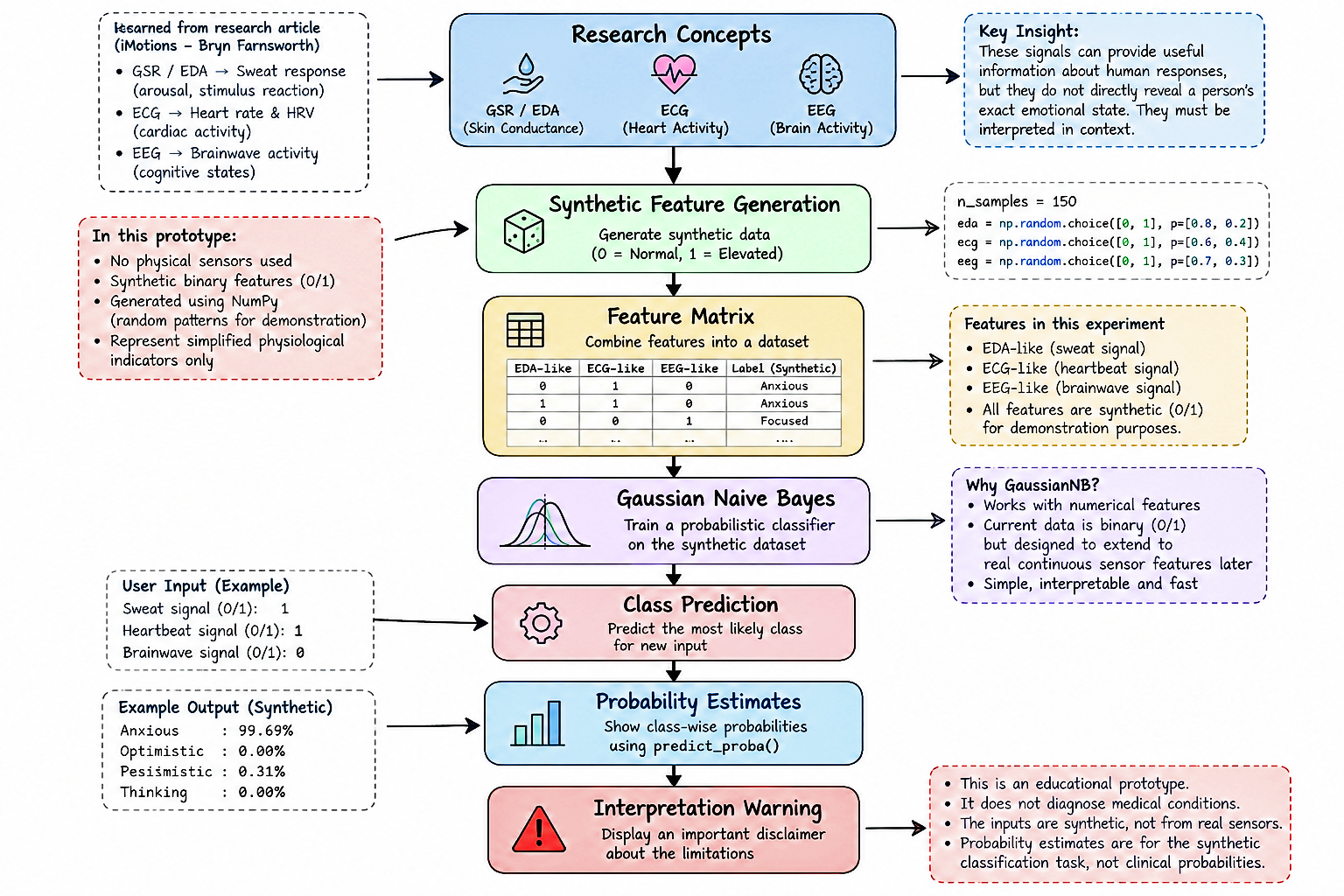
Figure 1: Conceptual pipeline illustrating the transition from research concepts to computational classification using synthetic physiological features.
2. The Engineering Decision: Why Gaussian Naive Bayes? ⚙️
Once the idea became concrete, I needed a classifier. I chose Gaussian Naive Bayes (GaussianNB) from Scikit-learn for this experimental version.
To understand that choice, we need to look at the mathematics—and the trade-off in using it with binary data.
2.1 A Quick Refresher on Bayes’ Theorem
Bayes’ Theorem describes how to update the probability of a hypothesis after observing evidence:
[ P(H\mid E)=\frac{P(E\mid H)P(H)}{P(E)} ]
Where:
(P(H)) is the prior probability of a hypothesis.
(P(E\mid H)) is the likelihood of observing the evidence under that hypothesis.
(P(E)) is the evidence, or the overall probability of observing it.
(P(H\mid E)) is the posterior probability after considering the evidence.
In classification, we want to estimate which class best explains an observed feature vector. Let the input be:
[ X=[x_1,x_2,x_3] ]
In this experiment, the three inputs stand in for simplified EDA-, ECG-, and EEG-inspired features.
Naive Bayes uses a simplifying assumption that features are conditionally independent given the class. Under that assumption:
[ P(C\mid X)\propto P(C)\prod_{i=1}^{n}P(x_i\mid C) ]
The proportionality symbol matters: class scores are normalized to obtain posterior estimates.
The conditional-independence assumption is a modelling convenience, not a statement about the human body. Real physiological signals can be correlated. Even so, Naive Bayes is a useful, lightweight way to explore probabilistic classification.
2.2 GaussianNB vs. BernoulliNB
Scikit-learn provides multiple Naive Bayes variants for different feature representations. Two relevant options are Gaussian Naive Bayes and Bernoulli Naive Bayes. See the official scikit-learn Naive Bayes documentation.
| Property | Gaussian Naive Bayes | Bernoulli Naive Bayes |
|---|---|---|
| Likelihood model | Gaussian distribution | Bernoulli distribution |
| Typical input | Numerical features modelled with a Gaussian likelihood | Binary or Boolean features |
| Main assumption | Each feature is approximately Gaussian within a class | Each feature represents a binary outcome |
| Potential role here | Experimenting with numerical sensor-derived features | A natural baseline for the current binary placeholders |
Gaussian Naive Bayes models the likelihood of a feature under a class using a Gaussian probability density function:
[ P(x_i\mid C=c)=\frac{1}{\sqrt{2\pi\sigma_{c,i}^{2}}}\exp\left(-\frac{(x_i-\mu_{c,i})^2}{2\sigma_{c,i}^{2}}\right) ]
Here:
(\mu_{c,i}) is the mean of feature (i) for class (c).
(\sigma_{c,i}^{2}) is the variance of that feature for the class.
(x_i) is the observed feature value.
These parameters are estimated from training data. The scikit-learn GaussianNB API reference documents this implementation.
2.3 The Trade-Off Behind My Choice
In my initial version, I used binary values—0 and 1—to keep synthetic data generation simple. But the broader direction I wanted to explore involved numerical measurements and features that might eventually be derived from sensor data.
A real feature could be a skin-conductance statistic, a cardiac measurement, or a summary statistic extracted from an EEG window. These values are not necessarily binary.
I therefore chose GaussianNB to experiment with a model family intended for numerical features under a Gaussian likelihood assumption. My intention was to keep a future numerical-feature path in mind.
However, there is an important caveat: GaussianNB is not automatically the best model for the binary data used here. BernoulliNB is specifically designed for binary features and is a natural baseline for this version. GaussianNB can be fitted to binary values, but doing so does not establish that its distributional assumptions fit the data well.
Likewise, real sensor-derived features are not guaranteed to follow Gaussian distributions. Future data could require other feature representations or models.
So this was a forward-looking experiment—not a proven performance advantage. A more rigorous next step is to compare GaussianNB and BernoulliNB on the same data split and report the results without overclaiming.
Choosing a classifier alone would not make the system sensor-ready. A real implementation would also require signal-specific preprocessing, feature extraction, appropriate labels, and validation on suitable data. The classifier is only one component of that larger pipeline.
3. Coding Against the Clock ⏱️
With enough of the research concepts understood to start experimenting, I moved into implementation. I did not have time to collect physiological recordings, build a hardware interface, or create a full signal-processing system.
Instead, I concentrated on the core computational workflow:
Generate synthetic features.
Create illustrative target labels.
Split the samples into training and test sets.
Train a Gaussian Naive Bayes model.
Evaluate predictions on held-out synthetic samples.
Accept new synthetic feature values and inspect the model output.
Display a warning explaining the limits of the experiment.
The warning was a deliberate part of the output. A model can return a confident-looking result even when the data and assumptions do not justify a real-world conclusion. I wanted the interface to make that distinction visible.
4. Building a Synthetic Classification Dataset
Synthetic data offered a practical way to test the programming workflow without collecting physiological measurements.
The following snippet generates binary placeholders for three feature channels:
import numpy as np
import pandas as pd

# Reproducible synthetic data generation
rng = np.random.default_rng(42)
n_samples = 600

data = pd.DataFrame({
    "eda_flag": rng.choice([0, 1], size=n_samples, p=[0.65, 0.35]),
    "ecg_flag": rng.choice([0, 1], size=n_samples, p=[0.60, 0.40]),
    "eeg_flag": rng.choice([0, 1], size=n_samples, p=[0.55, 0.45]),
})

print(data.head())
The names are only reminders of the concepts that inspired the features:
eda_flag: a simulated EDA-related indicator.ecg_flag: a simulated cardiac-related indicator.eeg_flag: a simulated EEG-related indicator.
These are not actual measurements. The probabilities are illustrative and do not come from physiological studies or measured population distributions.
Generating random numbers under names inspired by real sensors does not make the data physiologically realistic. The purpose here is to test the code and data pipeline—not to model the human body.
5. Training and Evaluating the Model
A supervised classifier needs target labels. For this example, I used simple rules to assign illustrative labels based on the generated features.
def assign_synthetic_label(row):
    """Assign an illustrative label from synthetic features.

    These are arbitrary demonstration rules—not a validated model
    of human emotion, attention, or psychological state.
    """
    eda = row["eda_flag"]
    ecg = row["ecg_flag"]
    eeg = row["eeg_flag"]

    if eda == 1 and ecg == 1:
        return "Elevated_Arousal_Proxy"
    if eeg == 1 and eda == 0:
        return "Attention_Like_Proxy"
    return "Baseline_Like_Proxy"


y = data.apply(assign_synthetic_label, axis=1)
print("Synthetic dataset created.")
print(y.value_counts())
Why use rules? They create a complete feature-and-label structure for experimenting with the classification pipeline. But there is a fundamental limitation: the target labels come from rules I defined myself. The model is learning patterns in an artificial labelling scheme; it is not discovering validated relationships between physiological signals and psychological states.
The names Elevated_Arousal_Proxy, Attention_Like_Proxy, and Baseline_Like_Proxy are demonstration labels, not clinically established categories.
Now we can split the data, train the classifier, and inspect its predictions:
from sklearn.model_selection import train_test_split
from sklearn.naive_bayes import GaussianNB
from sklearn.metrics import accuracy_score, classification_report

X_train, X_test, y_train, y_test = train_test_split(
    data,
    y,
    test_size=0.20,
    random_state=42,
    stratify=y,
)

model = GaussianNB()
model.fit(X_train, y_train)

y_pred = model.predict(X_test)
accuracy = accuracy_score(y_test, y_pred)

print("=== AI SHADOW PROFILER ===")
print(f"Training samples: {len(X_train)}")
print(f"Testing samples:  {len(X_test)}")
print(f"Synthetic-label accuracy: {accuracy:.2%}")
print("\nClassification report:")
print(classification_report(y_test, y_pred, zero_division=0))
This is an initial evaluation of the model on held-out samples from the same synthetic data-generating process. It is not a measurement of accuracy on real human emotions or psychological traits.
There is a subtle reason why toy datasets can produce surprisingly high scores: labels are generated directly from the input features, and only a small number of unique binary feature combinations are possible. The same combinations can appear in both the training and test sets. The evaluation therefore checks whether the classifier reproduces the artificial rules—not whether it generalizes to real physiology.
A more rigorous experiment would need an explicit research question, appropriately collected and labelled data, careful train/test separation, and validation independent of the modelling process. Comparing GaussianNB with BernoulliNB, inspecting a confusion matrix, analysing errors, and checking probability calibration would also make the evaluation more informative.
A numerical score is a starting point for investigation—not a substitute for it.
6. The Interactive Layer and Clinical Warning
A working model is one part of a project. Presenting its output clearly is another.
I wanted the experiment to accept input values, show the predicted synthetic class, and display the model's class-score estimates. The following minimal interactive example runs after the data and training snippets above:
print("\n=== AI SHADOW PROFILER: LIVE DEMO ===")

feature_names = ["eda_flag", "ecg_flag", "eeg_flag"]
values = []

for feature in feature_names:
    while True:
        try:
            value = int(input(f"Enter {feature} (0 or 1): "))
            if value in (0, 1):
                values.append(value)
                break
            print("Please enter either 0 or 1.")
        except ValueError:
            print("Invalid input. Enter an integer: 0 or 1.")

sample = pd.DataFrame([values], columns=feature_names)
predicted_label = model.predict(sample)[0]
probabilities = model.predict_proba(sample)[0]

print("\n=== EXPERIMENTAL CLASSIFICATION RESULT ===")
print(f"Predicted synthetic class: {predicted_label}")
print("\nModel score estimates:")

for label, probability in zip(model.classes_, probabilities):
    print(f"{label}: {probability:.2%}")

print("\n" + "=" * 55)
print("CLINICAL AND INTERPRETATION WARNING")
print("=" * 55)
print(
    "This is an educational machine learning prototype. It does not "
    "diagnose medical conditions, measure actual emotions, or establish "
    "personality traits."
)
print(
    "The current inputs are synthetic binary placeholders, not recordings "
    "from physiological sensors."
)
print(
    "The displayed scores describe the model's synthetic classification task; "
    "they are not clinical probabilities."
)
6.1 Why Include a Warning in the Output?
A label can sound more authoritative than the evidence behind it. For example, Attention_Like_Proxy may sound like a measurement of attention, but the name does not make it a scientifically validated metric.
Similarly, predict_proba() returns model-derived estimates. It does not independently establish that those estimates are calibrated, or that the predicted class corresponds to a genuine psychological state.
The warning is therefore part of the design—not an optional afterthought. It helps distinguish a computational prediction from a real-world conclusion.
7. What the Experiment Actually Demonstrated
Looking back, the most interesting part was not any single line of Python. It was the process of turning a question into an experiment.
The lab session gave me a starting point in Bayes’ Theorem. The psychophysiology article helped me think about measurable responses. Python and Scikit-learn gave me tools to express a simplified version of that idea computationally.
| Component | What the experiment explored |
|---|---|
| Probability theory | The intuition behind Bayesian inference |
| Synthetic data | Representing simplified features in a dataset |
| Classification | Training a Gaussian Naive Bayes model |
| Evaluation | Testing predictions on held-out synthetic samples |
| Interactive inference | Accepting feature values and displaying predictions |
| Responsible output | Distinguishing model estimates from psychological conclusions |
The professor's response gave me a reason to preserve the work and continue developing it. When I couldn't transfer the notebook from the college computer, I rewrote the implementation at home so I could keep experimenting.
That experience also reminded me of a practical engineering lesson: being able to reconstruct an idea is useful, but a reliable development workflow matters too. For future iterations, I want to use version control, separate data-generation code from training code, record experiment configurations, and make the pipeline reproducible.
Those improvements are just as important as adding new model features.
8. What Comes Next? From an Experiment to a More Rigorous System 🚀
AI Shadow Profiler is an early-stage experimental prototype. The synthetic dataset helps test the structure of a machine learning pipeline, but it does not validate the system for studying actual human behavior.
The next steps should address that gap rather than simply making the interface look more impressive.
8.1 Compare the Model Choices
I want to compare GaussianNB and BernoulliNB under the same experimental conditions. That would help determine which classifier is better suited to the current binary representation instead of assuming that a model chosen with future numerical inputs in mind is automatically the best option now.
The comparison should use the same data split and appropriate metrics, with results reported transparently.
8.2 Introduce Real Numerical Features Carefully
Real physiological sensing requires more than replacing zeros and ones with floating-point values. A genuine implementation would need to consider:
How signals are acquired and whether the recordings are reliable.
Which features are extracted from each signal.
How artifacts, missing values, and noisy recordings are handled.
Whether the model's statistical assumptions fit the measured features.
Whether differences between participants or recording conditions affect results.
The model choice would need to be revisited with the resulting data. Continuous measurements do not automatically follow Gaussian distributions, and model selection should be guided by evidence rather than a desire to future-proof the architecture in name only.
8.3 Define and Validate the Research Question
Before claiming that a model can classify emotions or behavioral states, the target must be defined and measured appropriately. That involves deciding what counts as the target state, how labels are established, how uncertainty is represented, and how the model will be tested outside the development dataset.
Physiological signals can provide useful evidence about some responses, but interpretation requires appropriate context and validation. A systematic review of machine learning for EDA-based arousal classification details the importance of acquisition, preprocessing, feature extraction, and model evaluation (review article).
8.4 Make the System Explainable and Privacy-Aware
Any future version should distinguish what the model observed, what it inferred, and what remains uncertain. It should also handle physiological information responsibly, using informed consent, data minimization, and appropriate safeguards.
The objective should not be to assign definitive psychological labels to people. It should be to investigate whether carefully defined models can provide useful and validated information about specific patterns under controlled conditions.
That is a much more meaningful engineering challenge.
Conclusion: One Experiment at a Time ⚡
AI Shadow Profiler began with a question during a college lab session.
I explored unfamiliar research concepts, translated some of their intuition into a simplified computational representation, experimented with Bayesian classification, and built an initial Python prototype.
The process was fast, imperfect, and constrained by the resources available. It also showed me how much more there is to investigate.
The current model does not read minds, diagnose conditions, or establish a person's emotional state. Its synthetic data lets me explore the mechanics of a classification pipeline, but further research and validation would be necessary before making real-world claims.
For me, that is part of the value of the experiment.
Engineering isn't just about getting code to run. It is also about understanding the assumptions behind it, examining what the results mean, and identifying what needs to improve next.
A classroom concept gave me the mathematical starting point. Independent research helped me develop an intuition. Implementation turned that intuition into something I could test.
Now, the next phase is to make the experiment more rigorous.
Understand the concept. Build the experiment. Question the result. Improve the system.
One experiment at a time.
Jai Maa Saraswati. 🙏
📌 Key Takeaway
AI Shadow Profiler is an experimental exploration of Bayesian classification using synthetic physiological features. Its current purpose is to investigate a computational pipeline—not to make validated claims about real human emotions or psychology.
The most important lesson from the 100-minute sprint is that a useful prototype is not the end of the engineering process. It is the beginning of more rigorous experimentation.
References and Further Reading 📚
Bryn Farnsworth, iMotions — Understanding Human Behavior – A Physiological Approach. The article that inspired the initial exploration of biosensors and physiological responses.
Scikit-learn — Naive Bayes. Official documentation covering Gaussian, Bernoulli, and other Naive Bayes variants and their assumptions.
Scikit-learn — GaussianNB API reference. Reference documentation for the Gaussian Naive Bayes classifier.
National Institute of Mental Health — Behavioral Assessment Methods for RDoC Constructs. Background on assessment methods and the interpretation of physiological measures.
Machine Learning Techniques for Arousal Classification from Electrodermal Activity: A Systematic Review. A review of signal acquisition, preprocessing, feature extraction, and machine learning in EDA-based arousal research.
Follow the Journey 🔗
GitHub: CODERUDRA-X
The AI Shadow Profiler repository is not being linked yet. I'll share a separate implementation update once the code, documentation, and project structure are ready to publish.
Tags: Artificial Intelligence · Machine Learning · Python · Bayesian Inference · Scikit-learn · Engineering Storytelling
About the author
- AI Research Engineer | Focus: AI & Defense Tech. Building high-stakes, decentralized multi-agent systems and safety-critical autonomous infrastructures for national defense capabilities. Creator of Aegis Swarm, NAAD and DataSentinal AI. Specialized in low-latency computer vision pipelines, edge-computing optimization, and sovereign open-source engineering.
Comments
Join the discussionNo comments yet. Be the first to comment.
